Stochastics | Mathematics Prelims

December 23, 2008

Periodicity, Positive Recurrence and Null Recurrence

Filed under: Stochastics — cjohnson @ 12:25 am

Imagine a chain where we start in some state (call it state zero), and the probability of being in state zero after $n$ transitions is zero unless $n$ is a multiple of some number, say $d$ . If $d$ is the smallest such number, then we say that that state has period $d$ . We’ve already seen an example of a chain with such a state in the simple random walk. In the simple random walk it was impossible to move from any state back to itself in an odd number of transitions: to do so you have to step left the same number of times you step right, which is of course an even number. Since two divides every even number, we have that the state has a period of two. A state with period one is called aperiodic.

If a state is recurrent, we say that the state is positive recurrent if the expected amount of time between recurrences (when the chain is in that state) is finite. A state that is recurrent but not positive recurrent is called null recurrent. A positive recurrent, aperiodic state is called ergodic.

An example of a null recurrent state appears in the simple random walk. We’ve seen that all states are recurrent, but it turns out that all states are in fact null recurrent. For a discussion of the null recurrence of states in the simple random walk, see section 2.2 in The Theory of Stochastic Processes by Cox and Miller.

December 22, 2008

Recurrence of States

Filed under: Probability Theory,Stochastics — cjohnson @ 9:25 pm

For some states in a Markov chain, there is a positive probability that once the chain transitions out of that state, it will never come back. For instance, in the chain with transition matrix

$\displaystyle \left[ \begin{array}{cc} 0 & 1 \\ 0 & 1 \end{array} \right]$

Once the chain transitions out of state one, it will never again enter state one, as it will stay in state two forever. There are times, however, when the chain will (with probability one) re-enter that state. For example, consider the chain

$\displaystyle \left[ \begin{array}{cc} 1/2 & 1/2 \\ 1/2 & 1/2 \end{array} \right]$

We note that the probability the chain re-enters state one at time $n$ is given by $(1/2)^n$ as chain must stay in state two for $n-1$ transitions, each of which has probability $1/2$ , and then must finally transition to state one with probability $1/2$ . Now, the probability the state ever re-enters state one is the union of the events where it first enters at $n=1$ , or at $n=2$ , or $n=3$ , … These are all disjoint events, though, so we have

$\displaystyle \sum_{n=1}^\infty \left(\frac{1}{2}\right)^n = 1$

We say that state $i$ is recurrent if, given $X_0 = i$ , the probability the chain will ever re-enter state $i$ is one. If a state is not recurrent, it is called transient. If a state is recurrent, then it will (with probability one) be entered infinitely often, assuming it’s entered at all, as the chain essentially “restarts” itself each time it enters that state, due to the Markov property.

Now suppose states $i$ and $j$ belong to the same class and that state $i$ is recurrent. Since $i$ and $j$ belong to the same class, we have $P_{ij} > 0$ . Note that $1 - P_{ij}$ (the probability of not transitioning to state $j$ from state $i$ ) is less than one. Each time the chain is in state $i$ there is a chance it will not transition to state $j$ . However, since $i$ is recurrent, it will be entered infinitely often, so the chance of never entering state $j$ is

$\displaystyle \prod_{n=1}^\infty (1 - P_{ij}) = 0$

So, if the chain enters state $i$ , it will (with probability one) also enter state $j$ at some point. This shows that if $i$ is recurrent, then $j$ must be as well. This shows that recurrence (and transcience) is a class property: in any given class, all states are transient or all states are recurrent.

An easier way to test for recurrence is to note that state $i$ is recurrent if and only if

$\displaystyle \sum_{n=1}^\infty P_{ii}^{(n)} = \infty$

(This follows by setting $I_n$ to be the Bernoulli random variable that is one if $X_n = i$ and zero otherwise. This expected number of times state one is entered is infinite, so $\mathbb{E}\left[\sum I_n \right]$ is infinite. By linearity, though, this expectation is simply $\sum \mathbb{E}[I_n] = \sum P_{ii}^{(n)}$ .)

Consider the simple random walk where the probability of stepping to the left or right at each transition is 1/2. We will suppose that our states are the integers, like we’re walking along an axis, and that we start in state zero. Note that all states communicate with all other states, so the chain is irreducible (there is only one class of states).

Now, supposing we’re in state zero, what’s the probability we ever re-enter state zero? To enter state zero, we must have had the same number of steps left as right. This is binomially distributed, so the probability that $X_n = 0$ is

$\displaystyle \binom{n}{n/2} \left(\frac{1}{2}\right)^{n/2} \left(\frac{1}{2}\right)^{n/2}$

Of course, this depends on $n$ being even, so we can rewrite this as

$\displaystyle P_{00}^{(2n)} = \binom{2n}{n} \left( \frac{1}{2} \right)^{2n}$

Using Stirling’s approximation to the factorial, re-writing the above binomial, we have that

$\displaystyle P_{00}^{(2n)} \sim \frac{4^n}{\sqrt{\pi n}}$

and so summing over all $n$ we have that $\sum P_{00}^{(2n)} = \infty$ which implies zero is a recurrent state. This in turn implies all states are recurrent.

December 20, 2008

Communication and Equivalence of States

Filed under: Probability Theory,Stochastics — cjohnson @ 4:41 pm

When states $i$ and $j$ , $i \neq j$ , of a Markov chain can be reached from one another (that is, there is a positive probability of transitioning to $i$ from $j$ , and a positive probability of transitioning to $j$ from $i$ ; note these needn’t be one-step transitions), we say that the two states communicate. Note that every state communicates with itself, as if we’re in state $i$ we’ll be in state $i$ after zero transitions. Communication of states forms an equivalence relation, and so when we say two states belong to the same class, we mean that they belong to the same equivalence class with this relation. If a chain has only one class of states, the chain is called irreducible.

For instance, consider the chain that simply moves from state one to state two, from state two to state three, then from state three back to state one, and the process repeats. Such a chain would have a transition probability matrix of

$\displaystyle \left[ \begin{array}{ccc} 0 & 1 & 0 \\ 0 & 0 & 1 \\ 1 & 0 & 0 \end{array} \right]$

This chain has only one class and so is irreducible.

The chain with transition matrix

$\displaystyle \left[ \begin{array}{cccc} 1/2 & 1/4 & 1/4 & 0 \\ 0 & 1/2 & 1/2 & 0 \\ 1/3 & 1/3 & 0 & 1/3 \\ 0 & 0 & 0 & 1 \end{array}\right]$

has two classes, $\{1, 2, 3\}$ and $\{4\}$ . The first three states communicate with one another as if you’re any one of $\{1, 2, 3\}$ , then there is a positive probability of transitioning to any of $\{1, 2, 3\}$ . Notice that we can transition from state two to state one by going through state three first. State four is in a class by itself, though, as state four can only communicate with itself: Once you’re in state four, you stay in state four with probability one.

The Chapman-Kolmogorov Equations

Filed under: Probability Theory,Stochastics — cjohnson @ 12:46 pm

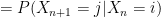
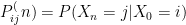
Supposing we’re given each $P_{ij}$ for a Markov chain, we have all of the one-step transition probabilities. Calculating the $n$ -step transition probabilities, we arrive at the Chapman-Kolmogorov equations. We will let $P_{ij}^(n)$ denote the probability that we arrive at state $j$ after $n$ transitions, given that we start in $i$ :

$\displaystyle P_{ij}^(n) = P(X_n = j | X_0 = i)$

We begin by considering $n = 2$ . If $X_0 = i$ , we find the chance of $X_2 = j$ by considering all the paths that start at $i$ and end at $j$ ; that is, we look at all posibilities of $X_1$ . Since we have each $P_{ik}$ , we just look at the chance we first transition to state $k$ , then from $k$ transition to $j$ . This gives

$\displaystyle P_{ij}^(2) = \sum_k P(X_2 = j \cap X_1 = k | X_0 = i)$

$\displaystyle \, \, = \sum_k P(X_2 = j| X_1 = k) P(X_1 = k | X_0 = i)$

$\displaystyle \, \, = \sum_k P(X_1 = j | X_0 = k) P(X_1 = k | X_0 = i)$

$\displaystyle \, \, = \sum_k P_{kj} P_{ik}$

$\displaystyle \, \, = \sum_k P_{ik} P_{kj}$

Note this gives the two-step transition probabilities form the matrix $P^2$ . We can extend this result inductively, then we have that the $n$ -step transition probability matrix is simply $P^n$ .

Continuing with the weather example from last time, we have that the two-step probability transition matrix is

$\displaystyle \left[ \begin{array}{ccc} 1/2 & 1/4 & 1/4 \\ 1/8 & 1/2 & 3/8 \\ 1/4 & 0 & 3/4 \end{array} \right]^2 = \left[ \begin{array}{ccc} 11/32 & 1/4 & 13/32 \\ 7/32 & 9/32 & 1/2 \\ 5/16 & 1/16 & 5/8 \end{array}\right]$

And so, according to our model, if it’s rainy today, there is an 11/32 chance it will be rainy two days from now, 1/4 chance it snows two days from now, and 13/32 chance it’s sunny.

Comments (1)

Introduction to Markov Chains

Filed under: Probability Theory,Stochastics — cjohnson @ 11:15 am

A stochastic process is an indexed collection of random variables, where the index is normally thought of as time. Generally we will assume that this time index is either discrete (i.e., from the set $\mathbb{N}$ or $\mathbb{N}_0$ ) or continous ( ${}[0, \infty)$ ). A Markov chain, unless stated otherwise, we will assume to be a discrete time process indexed by $\mathbb{N}_0$ . This is a process where each $X_n$ is a random variable whose range is a countable set, which we will generally take to be $\mathbb{N}$ or the first however-many natural numbers. We then say that $X_n$ is the state of the process at time $n$ , and the range of the $X_n$ is called the state space.

The primary property of a Markov chain is called the Markov property which effectively says that the distribution of $X_{n + 1}$ , given $X_n$ does not depend on any of $X_0, X_1, ..., X_{n-1}$ . That is, the next state we transition to depends only on the current state, and none of the previous. Formally,

$\displaystyle P(X_{n + 1} = j | X_n = i, X_{n-1} = i_{n-1}, X_{n-2} = i_{n-2}, ..., X_0 = i_0)$

$\displaystyle = P(X_{n+1} = j | X_n = i)$

For example, imagine that you were to start flipping a coin and you record the number of heads you get as you flip the coin, where each time you flip a head you add one to your total, but you subtract one each time you flip a tail. That is, if you were to flip HHTHTT your total would be zero. This is an example of a Markov chain because the probability your total after the next flip depends only what your total currently is, and not the “path” you took to get to that total. In our example, the probability we have one at the next flip is 1/2 (we flip heads) and the probability we have negative one at the next flip is 1/2 (we flip tails). This is also true if we were to flip HT or TTTTTTHHHHHH or any other string of heads and tails with the same number of heads as tails. A process such as the one we’ve described is called a random walk.

Because of this Markov property, we can describe the probability of transitioning between states as a matrix. Starting off with an example with finitely many states, suppose that if it’s raining today it will rain tomorrow with probability 1/2, snow with probability 1/4, or be sunny with probability 1/4. If it’s snowing today, it will rain tomorrow with probaiblity 1/8, snow with probability 1/2, and it will be sunny with probability 3/8. If it’s sunny today, it will rain tomorrow with probability 1/4, snow with probability 0, and be sunny with probability 3/4. The probability transition matrix is then

$\displaystyle \left[ \begin{array}{ccc} 1/2 & 1/4 & 1/4 \\ 1/8 & 1/2 & 3/8 \\ 1/4 & 0 & 3/4 \end{array} \right]$

Where, if we call this matrix $P$ , then the entry $P_{ij}$ refers to the probability that we transition to state $j$ , given that we’re in state $i$ . Also note that each row corresponds to a discrete probability distribution, so we must have that the sum of the entries on any given row is equal to one.

Comments (2)

Mathematics Prelims