Mathematics Prelims

December 1, 2009

Submodules and Homomorphisms

Filed under: Abstract Algebra,Algebra — cjohnson @ 8:57 pm

Just as a subgroup is a group within a group or a subfield is a field within a field, a submodule is a module within a module. That is, if $M$ is an $R$ -module, we say that $N$ is a submodule of $M$ if $N$ is a subgroup of $M$ and is closed under multiplication by elements of $R$ . This can be summarized by saying that for every $x, y \in N$ and every $r \in R$ , the following two properties hold.

$x - y \in N$
$rx \in N$

In the case of groups, we could only form a quotient group if the subgroup we were modding out by as sufficiently “nice” (i.e., was a normal subgroup); likewise, in the case of rings we required that a subring be nice (an ideal) in order to form a quotient ring. With modules however, we can always form the quotient module with a submodule. We can do this since, as $M$ is an abelian group under addition, all subgroups are normal and we can form the quotient group $M/N$ . This is naturally an abelian group, so in order to turn this into an $R$ -module we have to define multiplication of elements in $R$ and $M/N$ , which we do in the most obvious way: $r(x + N) = rx + N$ . To check that this is in fact an $R$ -module, we simply verify that the three axioms of a module hold.

$r((x + N) + (y + N)) = r(x + y + N) = r(x + y) + N = rx + ry + N = rx + N + ry + N$
$(r + s)(x + N) = (r + s)x + N = rx + sx + N = rx + N + sx + N$
$(rs)(x + N) = (rs)x + N = r(sx) + N = r(sx + N)$

Finally, if $M$ is a unitary module, then so too is $M/N$ : $1(x + N) = 1x + N = x + N$ .

We say a map $\phi : M \to N$ between two $R$ -modules is a homomorphism if $\phi$ is a group homomorphism with the additional property that for each $r \in R$ , $\phi(rx) = r \phi(x)$ . As you would expect, the kernel of this homomorphism is a submodule of $M$ , and the image is a submodule of $N$ .

Supposing that $S \subseteq M$ , we define $R\langle S \rangle$ to be the smallest submodule of $M$ containing $S$ , which is naturally the intersection of all submodules containing $S$

$\displaystyle R\langle S \rangle = \bigcap \left\{ N : N \text{ a submodule of } M \text{ and } S \subseteq N \right\}$

If $S$ is a finite set, we may write $R\langle s_1, s_2, \ldots, s_n \rangle$ in place of $R \langle S \rangle$ , and in the event that $S$ is a singleton, we say that $R\langle s_1 \rangle$ is a cyclic submodule of $M$ . We call the elements of $S$ the generating set of the $R \langle S \rangle$ submodule, and call the elements of $S$ the generators of this submodule.

Leave a Comment

November 28, 2009

Modules

Filed under: Abstract Algebra,Algebra — cjohnson @ 9:59 pm

Anyone who has spent any amount of time in algebra or analysis has come across vector spaces: a set of elements, vectors, which we can add together or multiply by a scalar from some fixed field. This idea is simple and natural enough that students in high-school physics classes become familiar with the basic idea of vectors, if only in an informal way. However, in the axioms of a vector space there’s nothing that particularly requires that we pull our scalars from a field (though other results in vector space theory depend on our having an underlying field). Indeed, we could just require that the scalars we multiply by simply be elements of a ring; this gives us a structure known as a module. Though this seems like a simple enough generalization, module theory has some quirks that those of us more accustomed to vector spaces will find odd. For instance, though every vector space has a basis, there are modules which do not; and even if a module has a basis, two different bases may have different cardinalities.

To be more precise, given a ring $R$ and an abelian group $M$ (written additively), we say that $M$ is a (left) $R$ -module if there exists a ring homomorphism $\phi : R \to \text{End}(M)$ . (Recall that if $M$ is an abelian group, the collection of endomorphisms of $M$ forms a ring under piecewise addition and function composition.) This says simply that given an $r \in R$ and an $x \in M$ , we can define the multiplication of $x$ by $r$ as $rx = \phi(r)(x)$ . Given any $r, s \in R$ and any $x, y \in M$ , the following are immediate consequences of our definition.

$(r + s)x = rx + sx$
$r(x + y) = rx + ry$
$(rs)x = r(sx)$

If in addition the ring $R$ has an identity, we may also require that $1x = x$ for all $x \in M$ . We call such a module unitary. Though this isn’t strictly required, we will assume that all modules we deal with are unitary if the ring has identity. Notice that we only perform multiplication on the left. If we define multiplication on the right, we have a right $R$ -module. We will assume that all of our modules are left module unless otherwise specified.

The three properties listed above aren’t simply consequences of our definition of a module, but can actually be used as an alternative definition. That is, if we have an abelian group $M$ , a ring $R$ , and some multiplication $R \times M \to M$ satisfying the above properties, we then have a module. To see this, define for each $r \in R$ a $M$ -endomorphism $\phi_r : M \to M$ by $x \mapsto rx$ . Notice that the second property above guarantees that $\phi_r$ is indeed an endomorphism: $\phi_r(x + y) = r(x + y) = rx + ry = \phi_r(x) + \phi_r(y)$ . Now defining a map $\phi : R \to \text{End}(M)$ as $r \mapsto \phi_r$ , properties one and three guarantee that this is in fact a ring homomorphism.

As stated earlier, a module can be thought of as a generalization of a vector space. In fact, if our ring $R$ is a field, then any $R$ -module is simply a vector space over $R$ . A module can also be thought of as a generalization of an abelian group, in the sense that every abelian group is in fact a $\mathbb{Z}$ -module. Suppose that $A$ is an abelian group. For each positive $n \in \mathbb{Z}$ , define $na$ as $\sum_{i=1}^n a$ . If $n = 0$ , define $na = 0$ . Finally, if $n < 0$ , define $na$ as the inverse (in $A$ ) of $(-n)a$ .

Notice that every ring can be viewed as a module over itself; $R$ is an $R$ -module where scalar multiplication is simply the ring’s usual multiplication. Additionally, if $S$ is a subring of $R$ , then $R$ can be viewed as an $S$ -module as the three properties of an $S$ -module are satisfied by usual multiplication in the ring. Similarly, if $I$ is left ideal of $R$ , then $I$ is a left $R$ -module; if $I$ is a right ideal, then it’s a right $R$ -module.

As we may pull our scalars from a ring instead of a field, we can treat some more “interesting” objects are scalars. For instance, suppose that $V$ is an $F$ -vector space and $T : V \to V$ a linear transformation. Then $F[x]$ , the set of all polynomials with coefficients from $F$ , forms a ring. For any $f(x) \in F[x]$ with $f(x) = \sum_{i=0}^n f_i x^i$ , we define $f(T) = \sum_{i=0}^n f_i T^i$ where $T^i$ means the $i$ -fold composition of $T$ with itself. For any $v \in V$ we define $f(x) \cdot v$ as $f(T)(v) = \sum_{i=0}^n f_i T^i(v)$ . Notice this satisfies the properties of a $F[x]$ -module.

$(f(x) + g(x)) \cdot v = (f(T) + g(T)) \cdot v = f(T)(v) + g(T)(v) = f(x) \cdot v + g(x) \cdot v$
$f(x) \cdot (u + v) = f(T)(u + v) = f(T)(u) + f(T)(v) = f(x) \cdot u + f(x) \cdot v$
$f(x) \cdot (g(x) \cdot v) = f(T)(g(T)(v)) = (f(T) \circ g(T))(v) = (f(T) g(T))(v) = (f(x) g(x)) \cdot v$

Thus this module, which we’ll denote $V_T$ , has polynomials as its scalars.

Leave a Comment

June 26, 2009

The Characteristic Polynomial

Filed under: Algebra,Linear Algebra — cjohnson @ 7:18 pm

Last time we defined the eigenvalues and eigenvectors of a matrix, but didn’t really discuss how to actually calculate the eigenvalues or eigenvectors; we said that if it so happened that your matrix was similar to a diagonal matrix, the non-zero entries of the diagonal matrix were the eigenvalues, and the columns of the change-of-basis matrix were the eigenvectors. Now we’re going to discuss how to find the eigenvalues using the matrix’s characteristic polynomial.

Notice that if $\lambda$ is an eigenvalue of $A$ with associated eigenvector $v$ we have the following.

$Av = \lambda v$

$\implies Av - \lambda v = 0$

$\implies (A - \lambda I) v = 0$

Of course, $v = 0$ satisfies this equation, but that’s a trivial solution. For any other, non-trivial, solution we’d require that $A$ is non-singular, and so $\text{det}(A - \lambda I) = 0$ . Thus if $\lambda$ is an eigenvalue of $A$ , we must have $\text{det}(A - \lambda I) = 0$ .

Now suppose that $\omega$ is such that $\text{det}(A - \omega I) = 0$ . Then there is a non-trivial solution to $(A - \omega I) u = 0$ , so $Au = \omega u$ , and $\omega$ is an eigenvalue. We’ve shown that $\lambda$ is an eigenvalue of $A$ if and only if $\text{det}(A - \lambda I) = 0$ . Furthermore, $\text{det}(A - \lambda I)$ is a polynomial in $\lambda$ (this is obvious if $A$ is $1 \times 1$ , and inductively we can show that this is true for $n \times n$ matrices). This means that with the characteristic polynomial, the problem of finding eigenvalues is reduced to finding the roots of a polynomial.

As an example, suppose

$\displaystyle A = \left[ \begin{array}{ccc} 1 & -1 & 2 \\ 2 & 2 & -3 \\ 3 & 5 & 7 \end{array} \right]$

Then the characterstic polynomial is

$\displaystyle \text{det} \left( \left[ \begin{array}{ccc} 1 - \lambda & -1 & 2 \\ 2 & 2 - \lambda & -3 \\ 3 & 5 & 7 - \lambda \end{array} \right] \right) = -\lambda^3 + 10\lambda^2 - 34 \lambda + 60$

$\displaystyle = -(\lambda-6) \, (\lambda^2 - 4 \lambda + 10)$

$\displaystyle = (\lambda - 6) \, (\lambda - (2 - i \sqrt{6})) \, (\lambda - (2 + i \sqrt{6}))$

So we see that the eigenvalues are $6$ , $2 - i \sqrt{6}$ , and $2 + i \sqrt{6}$ (notice the last two are complex conjugates of one another).

Now, once we’ve found the eigenvalues, the next step is to find the eigenvectors. Since

$Av = \lambda v$

$\implies (A - \lambda I) v = 0$

what we want is to find the nullspace of $A - \lambda I$ , since these are all the vectors that $A - \lambda I$ will take to zero. In our particular example, for $\lambda = 6$ ,

$(A - \lambda I) v = 0$

$\implies \left( \left[ \begin{array}{ccc} 1 & -1 & 2 \\ 2 & 2 & -3 \\ 3 & 5 & 7 \end{array} \right] - \left[ \begin{array}{ccc} 6 & 0 & 0 \\ 0 & 6 & 0 \\ 0 & 0 & 6 \end{array} \right] \right) \left[ \begin{array}{c} v_1 \\ v_2 \\ v_3 \end{array} \right] = 0$

$\implies \left[ \begin{array}{ccc} -5 & -1 & 2 \\ 2 & -4 & -3 \\ 3 & 5 & 1 \end{array} \right] \left[ \begin{array}{c} v_1 \\ v_2 \\ v_3 \end{array} \right] = 0$

Now we take the row-reduced echelon form of this matrix, since it shares the same null space:

$\implies \left[ \begin{array}{ccc} 1 & 0 & -\frac{1}{2} \\ 0 & 1 & \frac{1}{2} \\ 0 & 0 & 0 \end{array} \right] \left[ \begin{array}{c} v_1 \\ v_2 \\ v_3 \end{array} \right] = \left[ \begin{array}{c} 0 \\ 0 \\ 0 \end{array} \right]$

This tells us that

$\text{NS}(A - 6I) = \left\{ \left[ \begin{array}{c} \frac{1}{2} v_3 \\ -\frac{1}{2} v_3 \\ v_3 \end{array} \right] : v_3 \in \mathbb{C} \right\}$

So the eigenvectors associated with the eigenvalue $\lambda = 6$ are the multiples of $\left[ 0.5, \, -0.5, \, 1 \right]^T$ . We’d repeat the above process with $\lambda = 2 \pm i \sqrt{6}$ to find the other eigenvectors.

Comments (2)

June 25, 2009

Eigenvalues and Eigenvectors

Filed under: Algebra,Linear Algebra — cjohnson @ 2:39 pm

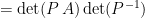
Let’s suppose that $A$ is an $n \times n$ matrix which is similar to a diagonal matrix, $\text{diag}(\lambda_1, \lambda_2, ..., \lambda_n)$ . This means there is an invertible (change-of-basis) matrix $P$ such that

$\displaystyle A = P \text{diag}(\lambda_1, ..., \lambda_n) P^{-1}$

Now since $P$ is a change of basis matrix, each of its columns gives the coordinates to a basis vector of some basis. Let’s call that basis $\beta$ and let $\beta_1$ through $\beta_n$ be the elements of that basis. Now, if we take the above equation and multiply by $P$ on the right, notice that

$AP = P \text{diag}(\lambda_1, ..., \lambda_n)$

$\implies (AP)_{*i} = (P \text{diag}(\lambda_1, ..., \lambda_n))_{*i} = \lambda_i P_{*i}$

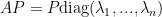
That is, the $i$ -th column of $AP$ is equal to the $i$ -th column of $P \text{diag}(\lambda_1, ..., \lambda_n)$ , which is just $\lambda_i$ times the $i$ -th column of $P$ . Since each column of $AP$ is just a linear combination of the columns of $A$ , though, we have

$AP_{*i} = \lambda_i P_{*i}$

This means that when we plug in the $i$ -th column of $P$ to the linear transformation represented by $A$ , we get back a multiple of that column. Calling the linear transformation $\tau$ , we have that

$\tau(\beta_i) = \lambda_i \beta_i$ .

Vectors such as $\beta_i$ whose image under $\tau$ is just a multiple of the vector are called eigenvectors of $\tau$ . That multiple, the $\lambda_i$ above, is called an eigenvalue of $\tau$ . These eigenvectors and eigenvalues are associated with a particular linear transformation, so when we talk about the eigenvectors and eigenvalues of a matrix, we really mean the eigenvectors and eigenvalues of the transformation represented by that matrix. Notice that this means that eigenvalues are independent of the chosen basis; since similar matrices represent the same transformation just with respect to different bases, similar matrices have the same eigenvalues.

We assumed that $A$ was similar to a diagonal matrix above, but this isn’t always true. If $A$ is similar to a diagonal matrix, say $A = P^{-1}DP$ , then as we’ve just shown, the columns of $P$ are eigenvectors of $A$ . Since these form the columns of a non-singular matrix, the eigenvectors of $A$ form a basis for the vector space. Also, if the eigenvectors of $A$ form a basis, let’s take those basis vectors as columns of $P$ .

$\displaystyle P^{-1} A P$

$\displaystyle = \left[ \begin{array}{c|c|c} \beta_1 & ... & \beta_n \end{array} \right]^{-1} A \left[ \begin{array}{c|c|c} \beta_1 & ... & \beta_n \end{array} \right]$

$\displaystyle = \left[ \begin{array}{c|c|c} \beta_1 & ... & \beta_n \end{array} \right]^{-1} \left[ \begin{array}{c|c|c} A \beta_1 & ... & A \beta_n \end{array} \right]$

$\displaystyle = \left[ \begin{array}{c|c|c} \beta_1 & \cdots & \beta_n \end{array} \right]^{-1} \left[ \begin{array}{c|c|c} \lambda_1 \beta_1 & \cdots & \lambda_n \beta_n \end{array} \right]$

$\displaystyle = \left[ \begin{array}{c|c|c} \beta_1 & \cdots & \beta_n \end{array} \right]^{-1} \left( \left[ \begin{array}{c|c|c} \beta_1 & \cdots & \beta_n \end{array} \right] \left[ \begin{array}{cccc} \lambda_1 & 0 & \cdots & 0 \\ 0 & \lambda_2 & \cdots & 0 \\ \vdots & & \ddots & \vdots \\ 0 & \cdots & 0 & \lambda_n \end{array} \right] \right)$

$\displaystyle = \text{diag}(\lambda_1, ..., \lambda_n)$

So a matrix is diagonalizable (similar to a diagonal matrix) if and only if its eigenvectors form a basis for the vector space.

Comments (4)

Definition of Similarity Using Linear Transformations

Filed under: Algebra,Linear Algebra — cjohnson @ 12:24 pm

Let’s suppose we have a linear transformation $\tau$ on $\mathbb{R}^3$ which performs the following:

$\displaystyle \left[ \begin{array}{c} 1 \\ 0 \\ 0 \end{array} \right] \mapsto \left[ \begin{array}{c} 1 \\ 2 \\ 3 \end{array} \right]$

$\displaystyle \left[ \begin{array}{c} 0 \\ 1 \\ 0 \end{array} \right] \mapsto \left[ \begin{array}{c} 4 \\ 5 \\ 6 \end{array} \right]$

$\displaystyle \left[ \begin{array}{c} 0 \\ 0 \\ 1 \end{array} \right] \mapsto \left[ \begin{array}{c} 5 \\ 7 \\ 0 \end{array} \right]$

Now, the matrix representation of this transformation with respect to the standard basis is clearly

$\displaystyle \left[ \begin{array}{ccc} 1 & 4 & 5 \\ 2 & 5 & 7 \\ 3 & 6 & 0 \end{array} \right]$

But suppose we were to use a different basis for $\mathbb{R}^3$ , like say $\zeta = \{ (2, 1, 0)^T, \, (1, 0, 1)^T, \, (3, 0, -1)^T \}$ . We see that our transformation maps these basis vectors as follows:

$\displaystyle \left[ \begin{array}{c} 2 \\ 1 \\ 0 \end{array} \right] \mapsto \left[ \begin{array}{c} 6 \\ 9 \\ 12 \end{array} \right]$

$\displaystyle \left[ \begin{array}{c} 1 \\ 0 \\ 1 \end{array} \right] \mapsto \left[ \begin{array}{c} 6 \\ 9 \\ 3 \end{array} \right]$

$\displaystyle \left[ \begin{array}{c} 3 \\ 0 \\ -1 \end{array} \right] \mapsto \left[ \begin{array}{c} -2 \\ -1 \\ 9 \end{array} \right]$

Notice that with the vectors we have on both the left and the right above are the coordinates with respect to the standard basis. We’d like to see what the matrix representing $\tau$ looks like with respect to the $\zeta$ basis, so let’s convert the vectors on the right to $\zeta$ -coordinates. Recalling that a change of basis is simply a system of equations where the columns of the coefficient matrix are the coordinates of the basis vectors (and the inverse of this matrix if we want to go the other way), we have that

$\displaystyle \left[ \begin{array}{c} 6 \\ 9 \\ 12 \end{array} \right] = \left[ \begin{array}{c} 9 \\ 6 \\ -6 \end{array} \right]_{\zeta}$

$\displaystyle \left[ \begin{array}{c} 6 \\ 9 \\ 3 \end{array} \right] = \left[ \begin{array}{c} 9 \\ -\frac{3}{4} \\ -\frac{15}{4} \end{array} \right]_{\zeta}$

$\displaystyle \left[ \begin{array}{c} -2 \\ -1 \\ 9 \end{array} \right] = \left[ \begin{array}{c} 19 \\ \frac{7}{4} \\ - \frac{5}{2} \end{array} \right]_{\zeta}$

So with respect to our $\zeta$ basis, the representation of $\tau$ is

$\displaystyle \left[ \begin{array}{ccc} 9 & 9 & 19 \\ 6 & -\frac{3}{4} & \frac{7}{4} \\ -6 & -\frac{15}{4} & -\frac{5}{2} \end{array} \right]$

We will denote this matrix as $_\zeta[\tau]_\zeta$ where the right-most subscript means that inputs are in $\zeta$ -coordinates, and the left-most subscript means the outputs are in $\zeta$ -coordinates as well. Note that we could calculate $_\zeta[\tau]_\zeta$ by going from $\zeta$ coordinates to standard coordinates, using the earlier matrix, then going back to $\zeta$ -coordinates. That is,

$\displaystyle _\zeta[\tau]_\zeta = _\zeta[I]_e \, _e[\tau]_e \, _e[I]_\zeta$

where $_e[I]_\zeta$ refers to the $\zeta$ -to-standard basis change of basis matrix. For notational convenience, define the following

$A := _\zeta[\tau]_\zeta$

$B := _e[\tau]_e$

$P := _e[I]_\zeta$

Then the above becomes

$A = P^{-1} \, B \, P$

Any matrices $A$ and $B$ for which there exists a $P$ with satisfying this equation are called similar matrices. Note that two matrices are similar if and only if they represent the same linear transformation, but with respect to different bases. Also note that every non-singular matrix represents a change of basis matrix. Similarity forms an equivalence relation on the set of square matrices / the set of linear transformations from a finite dimensional vector space to itself.

Leave a Comment

June 18, 2009

Linear Transformations and Matrix Representations

Filed under: Algebra,Linear Algebra — cjohnson @ 2:22 pm

A common theme in mathematics is (or seems to be) looking at sets with a particular structure, and then looking at functions between those sets which preserve that structure. In groups we have homomorphisms; in topological spaces we have continuous maps; in general categories we have morphisms. In the particular case of vector spaces, though, there are two particular “structures” we want to preserve: vector addition and scalar multiplication. The maps which preserve these are what we refer to as linear transformations.

Specifically, suppose $V$ and $W$ are vector spaces over the field $\mathcal{F}$ . A function $\tau : V \to W$ is called a linear transformation if for all scalars $\alpha, \beta \in \mathcal{F}$ and for all vectors $u, v \in V$ we have

$\displaystyle \tau(\alpha u + \beta v) = \alpha \tau(u) + \beta \tau(v)$

Note that because of this linearity, a linear transformation is completely determined by how it maps the basis vectors of the domain. Suppose that $\beta = \{ \beta_1, \beta_2, ..., \beta_n \}$ is a basis for V. Let $u$ be any vector in $V$ with $u = a_1 \beta_1 + ... + a_n \beta_n$ . We then have

$\tau(u) = \tau(a_1 \beta_1 + ... + a_n \beta_n) = a_1 \tau(\beta_1) + ... + a_n \tau(\beta_n)$ .

So if we know each $\tau(\beta_i)$ , we can figure out where any other vector will be sent by $\tau$ . This does not mean that $\tau(\beta_1), ..., \tau(\beta_n)$ is necessarily a basis for the range, $\tau(V)$ . It could be that $\tau(\beta_1) = \tau(\beta_2)$ , in which case these vectors are linearly dependent and can’t both be in the basis. We do have that $\tau(\beta_1), ..., \tau(\beta_n)$ span $\tau(V)$ , however, so as long as they’re linearly independent they’ll form a basis.

The main thing we want to notice about linear transformations for right now is that if both $V$ and $W$ are finite dimensional, then a linear transformation $\tau : V \to W$ can be represented as a matrix. Suppose that $V$ is $n$ -dimensional with the $\beta$ basis mentioned above, and that $W$ is $m$ -dimensional with basis $\omega = \{ \omega_1, ..., \omega_m \}$ . Note that the properties of matrix multiplication tell us that any $m \times n$ matrix defines a linear transformation from $V$ to $W$ :

$A(\alpha u + \gamma v) = A(\alpha u) + A( \gamma v) = \alpha A u + \gamma A v$

Now suppose $\tau : V \to W$ is any other linear transformation. Suppose that the coordinate vector of $\tau(\beta_i)$ with respect to the $\omega$ basis is

$\displaystyle \tau(\beta_i) = \left[ \begin{array}{c} a_{1i} \\ a_{2i} \\ \vdots \\ a_{mi} \end{array} \right]_\omega$

Now let $u = b_1 \beta_1 + ... + b_n \beta_n$ . We then have

$\displaystyle \tau(u)$

$\displaystyle \, = b_1 \tau(\beta_1) + b_2 \tau(\beta_2) + ... + b_n \tau(\beta_n)$

$\displaystyle \, = b_1 \left[ \begin{array}{c} a_{11} \\ a_{21} \\ \vdots \\ a_{m1} \end{array} \right] + b_2 \left[ \begin{array}{c} a_{12} \\ a_{22} \\ \vdots \\ a_{m2} \end{array} \right] + ... + b_n \left[ \begin{array}{c} a_{1n} \\ a_{2n} \\ \vdots \\ a_{mn} \end{array} \right]$

$\displaystyle \, = \left[ \begin{array}{cccc} a_{11} & a_{12} & \cdots & a_{1n} \\ a_{21} & a_{22} & \cdots & a_{2n} \\ \vdots & & & \vdots \\ a_{m1} & a_{m2} & \cdots & a_{mn} \end{array} \right] \left[ \begin{array}{c} b_1 \\ b_2 \\ \vdots \\ b_n \end{array} \right]$

Thus a linear transformation between finite dimensional vector spaces can be represented as a matrix. Notice that the entries of our matrix depend on our particular chosen bases: if one basis were altered, the matrix would change, even though the transformation is the same. We will denote the matrix representing $\tau$ with respect to the $\omega$ and $\beta$ bases as $_\omega[ \tau ]_\beta$

Leave a Comment

June 17, 2009

The Laplace/Cofactor Expansion

Filed under: Algebra,Linear Algebra — cjohnson @ 3:22 pm

We’ve yet to describe a way to calculate determinants in any easy way; we’ve seen some nice properties, but still have to resort to writing a non-elementary matrix as a product of elementary matrices in order to calculate its determinant. What we want to do now is describe a recursive procedure for calculating a determinant by looking at determinants of submatrices. 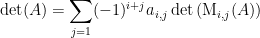Let’s first agree to call the submatrix of $A$ with the $i$ -th row and $j$ -th column deleted the $i,j$ –minor of $A$ , which we’ll denote $\text{M}_{i,j}(A)$ . So, supposing

$\displaystyle A = \left[ \begin{array}{ccc} 2 & 3 & 5 \\ 7 & 9 & 11 \\ 13 & 17 & 19 \end{array}\right]$

if we delete the first row and second column we have

$\displaystyle \text{M}_{1,2}(A) = \left[ \begin{array}{cc} 7 & 11 \\ 13 & 19 \end{array} \right]$

Let’s also note that if the first row of $A$ is all zeros except for the first entry, the determinant of $A$ is simply the determinant of $\text{M}_{1,1}(A)$ multiplied by that first entry. That is,

To see this, first note that we can zero out the entries in the first column below the $a_{11}$ by performing a sequence of elementary row operations that don’t change the determinant. Now we clearly have

$\displaystyle \det \left[ \begin{array}{c|ccc} a_{11} & 0 & \cdots & 0 \\ \hline a_{21} & & & \\ \vdots & & \text{M}_{1,1}(A) & \\ a_{n1} & & & \end{array} \right] = a_{11} \det \left[ \begin{array}{c|ccc} 1 & 0 & \cdots & 0 \\ \hline 0 & & & \\ \vdots & & \text{M}_{1,1}(A) & \\ 0 & & & \end{array} \right]$

Supposing we can write $\text{M}_{1,1}(A)$ as a product of elementary matrices, $\text{M}_{1,1}(A) = E_1 \, E_2 \, ... \, E_m$ , to calculate its determinant, we can then obtain the matrix above by looking at the product

$\displaystyle \left[ \begin{array}{cc} 1 & 0 \\ 0 & E_1 \end{array} \right] \, \left[ \begin{array}{cc} 1 & 0 \\ 0 & E_2 \end{array} \right] \, \cdots \, \left[ \begin{array}{cc} 1 & 0 \\ 0 & E_m \end{array} \right]$

Each of these is then an elementary matrix whose determinant is the same as the determinant of the associated $E_i$ matrix, so we have our result.

Now, applying the linearity we discussed last time,

$\displaystyle \det \left[ \begin{array}{ccc} a_{11} & \cdots & a_{1n} \\ & R_2 & \\ & \vdots & \\ & R_n & \end{array} \right] = \det \left[ \begin{array}{ccccc} a_{11} & 0 & \cdots & 0 & 0 \\ & & R_2 & & \\ & & \vdots & & \\ & & R_n & & \end{array} \right] + \det \left[ \begin{array}{ccccc} 0 & a_{12} & 0 & \cdots & 0 \\ & & R_2 & & \\ & & \vdots & & \\ & & R_n & & \end{array} \right] + ... + \det \left[ \begin{array}{ccccc} 0 & 0 & \cdots & 0 & a_{1n} \\ & & R_2 & & \\ & & \vdots & & \\ & & R_n & & \end{array} \right]$

Notice that we can can zero out the elements in the first column below $a_{11}$ giving us

$\displaystyle \det \left[ \begin{array}{ccccc} a_{11} & 0 & \cdots & 0 & 0 \\ & & R_2 & & \\ & & \vdots & & \\ & & R_n & & \end{array} \right] = a_{11} \det \left( \text{M}_{11}(A) \right)$

In general, for the $j$ -th column, we want to do a series of column swaps bringing the $j$ -th column to the front of the matrix, but keeping the other columns in order. (For this reason a single column swap won’t work, since that permutes the remaining columns.) Each time we swap columns, the determinant is multiplied by -1. If we move the $j$ -th column to the left by swapping with column $j-1$ , then with column $j-2$ , and so on, we perform $j-1$ swaps. Thus

$\det \left[ \begin{array}{ccccc} \cdots & 0 & a_{1j} & 0 & \cdots \\ & & R_2 & & \\ & & \vdots & & \\ & & R_n & & \end{array} \right] = (-1)^{j-1} \det \left[ \begin{array}{c|ccc} a_{1j} & 0 & \cdots & 0 \\ \hline 0 & & & \\ \vdots & & \text{M}_{1,j}(A) & \\ 0 & & & \end{array} \right] = (-1)^{j-1} a_{1j} \det \left( \text{M}_{1,j}(A) \right)$

So in total we have

$\displaystyle \det(A) = \sum_{j=1}^n (-1)^{j-1} a_{1,j} \det \left( \text{M}_{1,j}(A) \right)$

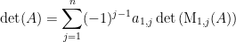
We could also perform this expansion along another row, but we’d have to perform some row swaps to move that row to the top first. Supposing we decide to expand along the $i$ -th row, we’ll perform $i-1$ swaps, each time multiplying the determinant by -1. We’d multiply our result above, then by $(-1)^{i-1}$ . Distributing that across our sum though, we note that

$(-1)^{i-1} \, (-1)^{j-1} = (-1)^{i + j - 2} = (-1)^{i + j} \, (-1)^{-2} = (-1)^{i + j}$

So, if we expand along the $i$ -th row, our formula becomes

$\displaystyle \det(A) = \sum_{j=1} (-1)^{i+j} a_{i,j} \det \left( \text{M}_{i,j}(A) \right)$

Each term of the sum with the $a_{i,j}$ factor removed is called a cofactor; The $i,j$ -th cofactor, which we’ll denote $\text{cof}_{i,j}(A)$ is

$\displaystyle \text{cof}_{i,j}(A) = (-1)^{i+j} \det \left( \text{M}_{i,j}(A) \right)$

The procedure we’ve just described is known as the Laplace expansion (or cofactor expansion) for the determinant, and so now we have a more efficient way of calculating determinants. (Notice that we could expand along a column instead of a row: just repeat the above procedure on the transpose of the matrix.)

Comments (3)

June 16, 2009

Determinants Are Linear in Rows and Columns

Filed under: Algebra,Linear Algebra — cjohnson @ 8:55 pm

One easy consequence of our definition of determinant from last time is that any singular matrix must have determinant zero. Suppose $A$ is a singular $n \times n$ matrix and that $P$ is the matrix which puts $A$ into row reduced form. Then we have

$\displaystyle \det(A)$

$\displaystyle = \det(P \, P^{-1} \, A)$

$\displaystyle = \det(P) \, \det(P^{-1}) \, \det(A)$

$\displaystyle = \det(P) \, \det(A) \, \det(P^{-1})$

$\displaystyle = \det(P \, A) \det(P^{-1})$

If $A$ is singular, once we put it in row reduced form it must have a row of zeros. We can now break $PA$ up into a product of elementary matrices, one of which will have be of the form $I_{(0R_i)}$ . We know that this matrix will have determinant zero, so the product will be zero, and thus $\det(A) = 0$ . Likewise, if $\det(A) = 0$ , we can write $A$ as a product of elementary row matrices and one will be $I_{(0R_i)}$ , so $A$ is singular. Now we know that a matrix is singular if and only if its determinant is zero.

Suppose now that the first row of $A$ can be written as $\alpha + \beta$ for some vectors $\alpha$ and $\beta$ . We wish to show that

$\displaystyle \det(A) = \det \left[ \begin{array}{c} \alpha + \beta \\ R_2 \\ \vdots \\ R_n \end{array} \right] = \det \left[ \begin{array}{c} \alpha \\ R_2 \\ \vdots \\ R_n \end{array} \right] + \det \left[ \begin{array}{c} \beta \\ R_2 \\ \vdots \\ R_n \end{array} \right]$

First suppose that the rows $R_2$ through $R_n$ form a linearly dependent set. Then our matrix is singular so has determinant zero. The determinants on the right in the above equation are zero too, so our we have our result.

Suppose now that $R_2$ through $R_n$ are linearly independent. We can then extend these to a basis for $\mathcal{F}_{1 \times n}$ by adding a vector, call it $\zeta$ . Then there exist scalars $a_i, b_i$ for $i = 1, ..., n$ such that

$\alpha = a_1 \zeta + a_2 R_2 + ... + a_n R_n$

$\beta = b_1 \zeta + b_2 R_2 + ... + b_n R_n$

Some simple manipulations from last time give us the following.

$\displaystyle \det \left[ \begin{array}{c} \alpha \\ R_2 \\ \vdots \\ R_n \end{array} \right]$

$\displaystyle = \det \left[ \begin{array}{c} a_1 \zeta + a_2 R_2 + ... + a_n R_n \\ R_2 \\ \vdots \\ R_n \end{array} \right]$

$\displaystyle = \det \left[ \begin{array}{c} a_1 \zeta \\ R_2 \\ \vdots \\ R_n \end{array} \right]$

$\displaystyle = a_1 \det \left[ \begin{array}{c} \zeta \\ R_2 \\ \vdots \\ R_n \end{array} \right]$

And likewise,

$\displaystyle \det \left[ \begin{array}{c} \beta \\ R_2 \\ \vdots \\ R_n \end{array} \right] = b_1 \det \left[ \begin{array}{c}\zeta \\ R_2 \\ \vdots \\ R_n \end{array} \right]$

Now we combine these results,

$\displaystyle \det \left[ \begin{array}{c} \alpha + \beta \\ R_2 \\ \vdots \\ R_n \end{array} \right]$

$\displaystyle = \det \left[ \begin{array}{c} (a_1 + b_1) \zeta + (a_2 + b_2) R_2 + ... + (a_n + b_n) R_n \\ R_2 \\ \vdots \\ R_n \end{array} \right]$

$\displaystyle = (a_1 + b_1) \det \left[ \begin{array}{c} \zeta \\ R_2 \\ \vdots \\ R_n \end{array} \right]$

$\displaystyle = a_1 \det \left[ \begin{array}{c} \zeta \\ R_2 \\ \vdots \\ R_n \end{array} \right] + b_1 \det \left[ \begin{array}{c} \zeta \\ R_2 \\ \vdots \\ R_n \end{array} \right]$

$\displaystyle = \det \left[ \begin{array}{c} \alpha \\ R_2 \\ \vdots \\ R_n \end{array} \right] + \det \left[ \begin{array}{c} \beta \\ R_2 \\ \vdots \\ R_n \end{array} \right]$

Since we can swap rows without altering the determinant, this result holds for any rows. A similar argument shows the result also holds for columns.

Comments (1)

June 13, 2009

Determinants

Filed under: Algebra,Linear Algebra — cjohnson @ 9:10 pm

I remember that when I took linear algebra, I had learned determinants in a very “algorithmic” sort of way; a determinant to me was a function defined on square matrices by a particular recursive procedure. In Charles Cullen’s Matrices and Linear Transformations, however, he defines a determinant not by a rule, but by two properties which completely characterize the determinant. A determinant, according to Cullen, is an $\mathcal{F}_{n \times n} \to \mathcal{F}$ function which satisfies the following.

For any two $n \times n$ matrices $A$ and $B$ , $\det(AB) = \det(A) \det(B)$
The determinant of $\text{diag}(k, 1, 1, ..., 1)$ is $k$ .

That’s it. That’s all you need to define the determinant. Of course, now we have to worry about whether a function with these properties even exists or not, and if so, is that function is unique? Before answering either of those questions, though, we need to establish that every $n \times n$ matrix can be written as a product of elementary matrices (where by an elementary matrix we mean one which results in an elementary row (or column) operation when multiplied on the left (or right), including zeroing out a row or column). To see this, recall that for every matrix $A$ there exist non-singular matrices $P$ and $Q$ such that

$\displaystyle PAQ = \left[ \begin{array}{cc} I_r & 0 \\ 0 & 0 \end{array} \right]$

where $r = \text{rank}(A)$ . In the above, $P$ represents a sequence of elementary row operations, and $Q$ gives a sequence of elementary column operations; $P$ and $Q$ are the products of elementary matrices. Since these are non-singular we have

$\displaystyle A = P^{-1} \left[ \begin{array}{cc} I_r & 0 \\ 0 & 0 \end{array} \right] Q^{-1}$

The middle matrix is clearly a product of matrices of the form $\text{diag}(1, ..., 1, 0, 1, ..., 1)$ . If we agree to also call such matrices elementary, then every square matrix is a product of elementary matrices.

Supposing we have a $\det$ function satisfying the properties given above, we can calculate the determinant of an elementary matrix pretty easily. In the following, $I_{(kR_i)}$ means we multiply the $i$ -th row by $k$ in the identity matrix; $I_{(R_i \leftrightarrow R_j)}$ means we swap rows $i$ and $j$ ; $I_{(kR_i + R_j)}$ means we add $k$ times row $i$ to row $j$ .

First we’ll look at scalar multiples of a particular row:

$\displaystyle \det\left( I_{(kR_i)} \right)$

$\displaystyle \, = \det\left( I_{(R_i \leftrightarrow R_1)} \, I_{(kR_1)} \, I_{(R_i \leftrightarrow R_j)} \right)$

$\displaystyle \, = \det \left( I_{(R_i \leftrightarrow R_1)} \right) \, \det \left( I_{(kR_1)} \right) \, \det \left( I_{(R_i \leftrightarrow R_1)} \right)$

$\displaystyle \, = \det \left( I_{(kR_1)} \right) \, \det \left( I_{(R_i \leftrightarrow R_1)} \right) \, \det \left( I_{(R_i \leftrightarrow R_1)} \right)$ (these are scalars in a field, so they commute)

$\displaystyle \, = \det \left( I_{(kR_1)} \right) \, \det \left( I_{(R_i \leftrightarrow R_1)} \, I_{(R_i \leftrightarrow R_1)} \right)$

$\displaystyle \, = \det \left( I_{(kR_1)} \right) \, \det \left( I \right)$

$\displaystyle \, = \det \left( I_{(kR_1)} \right)$

$\displaystyle \, = k$

Using similar identities we can show $\det \left( I_{(R_i \leftrightarrow R_j)} \right) = -1$ and $\det \left( I_{kR_i + R_j} \right) = 1$ . Now we know the determinants for all elementary matrices. Since every square matrix is a product of elementary matrices, and we can split the determinant up across a product of matrices, we can even calculate the determinant of any square matrix based solely on the two properties given earlier. (Note this isn’t necessarily an efficient way to calculate the determinant, just a possible way.)

At this point it shouldn’t seem too surprising that the two properties above are all we need to define a determinant: every square matrix is a product of elementary matrices, and we can “massage” elementary matrices into a form whose determinant we can calculate. In coming posts we’ll see how to expand this to define the Laplace / cofactor expansion for the determinant; the relationship between determinants and inverses; and Cramer’s rule, which tells us how to compute a single coordinate in the solution vector to a system of equations.

Comments (2)

Change of Basis

Filed under: Algebra,Linear Algebra — cjohnson @ 4:19 pm

In any non-trivial vector space there will be several possible bases we could pick. In $\mathbb{R}^3$ , for instance, we could use $\{ [1, 0, 0]^T, [0, 1, 0]^T, [0, 0, 1]^T \}$ or $\{ [1, 2, 0]^T, [3, 0, 1]^T, [4, 2, -1]^T \}$ . This first basis is known as the standard basis, and in general for an $n$ -dimensional vector space over $\mathcal{F}$ , we’ll refer to $\{ [1, 0, 0, ..., 0]^T, [0, 1, 0, ..., 0]^T, ..., [0, ..., 0, 1]^T \}$ as the standard basis, and will let $e_i$ denote the vector with a 1 in the $i$ -th position, and zeros elsewhere.

When we write down a vector like $[1, 2, 3]^T$ we implicitly mean that these are the coordinates to use with the vectors in the standard basis; these are the coefficients we multiply the $e_i$ basis vectors by to get describe our vector.

$\displaystyle \left[ \begin{array}{c} 1 \\ 2 \\ 3 \end{array} \right] = 1 \left[ \begin{array}{c} 1 \\ 0 \\ 0 \end{array} \right]+ 2 \left[ \begin{array}{c} 0 \\ 1 \\ 0 \end{array} \right] + 3 \left[ \begin{array}{c} 0 \\ 0 \\ 1 \end{array} \right]$

But how would we find the appropriate coordinates if we were to use $\{ [1, 2, 0]^T, [3, 0, 1]^T, [4, 2, -1]^T \}$ as our basis? Let’s suppose our coefficients are $\alpha_1, \alpha_2, \alpha_3$ . Then what we want to do is find the values of the $\alpha_i$ such that

$\displaystyle \alpha_1 \left[ \begin{array}{c} 1 \\ 2 \\ 0 \end{array} \right] + \alpha_2 \left[\begin{array}{c}3 \\ 0 \\ 1\end{array}\right] + \alpha_3\left[\begin{array}{c}4 \\ 2 \\ -1\end{array}\right] = \left[ \begin{array}{c} 1 \\ 2 \\ 3 \end{array}\right]$

So what we have is a system of equations:

$\displaystyle \left[ \begin{array}{ccc} 1 & 3 & 4 \\ 2 & 0 & 2 \\ 0 & 1 & -1 \end{array} \right] \left[ \begin{array}{c} \alpha_1 \\ \alpha_2 \\ \alpha_3 \end{array} \right]= \left[ \begin{array}{c} 1 \\ 2 \\ 3 \end{array} \right]$

Notice that since the columns of this matrix form a basis for $\mathbb{R}^3$ , the matrix is invertible, and so we can easily solve for the $\alpha_i$ .

$\displaystyle \left[ \begin{array}{c} \alpha_1 \\ \alpha_2 \\ \alpha_3 \end{array} \right] = \left[ \begin{array}{ccc} 1 & 3 & 4 \\ 2 & 0 & 2 \\ 0 & 1 & -1 \end{array} \right]^{-1} \left[ \begin{array}{c} 1 \\ 2 \\ 3 \end{array} \right] = \left[ \begin{array}{c} 5/2 \\ 3/2 \\ -3/2\end{array} \right]$

In general, if we have a basis $A = \{ a_1, ..., a_n \}$ , we will write

$\displaystyle \left[ \begin{array}{c} \alpha_1 \\ \vdots \\ \alpha_n \end{array} \right]_A$

to mean that the $\alpha_i$ are the coefficients of the $a_i$ vectors in our $A$ basis, and will let $_AI$ be the matrix converts the coordinates for the standard basis to coordinates in our $A$ basis. Likewise, $I_A$ will be the matrix which converts coordinates from the $A$ basis to coordinates with the standard basis.

Generalizing on the argument above we see that we can calculate $I_A$ by simply using our basis vectors as our columns. For $_AI$ we take the inverse of this matrix.

$\displaystyle I_A = \left[ \, \left. a_1 \, \right| \, \left. a_2 \, \right| \, \left. \cdots \, \right| \, a_n \, \right]$

$\displaystyle _AI = \left[ \, \left. a_1 \, \right| \, \left. a_2 \, \right| \, \left. \cdots \, \right| \, a_n \, \right]^{-1}$

Now suppose we have two bases, $A = \{ a_1, ..., a_n \}$ and $B = \{ b_1, ..., b_n \}$ . The matrix which will take coordinates with respect to the $A$ basis and convert them into coordinates for the $B$ basis is denoted $_BI_A$ . One way to calculate $_BI_A$ is to convert our $A$ -coordinates into standard coordinates, and then convert those into $B$ -coordinates: