If  is a probability space and
  is a measurable space (i.e., a set
  along with a sigma-algebra
  on ), then a random variable is a measurable function
  . That is, for each
  , we have
  . Generally speaking, we’ll be taking to be
  where
where  is the Borel algebra on
  .
.
Given a topological space  , there exists a sigma-algebra
  , called the Borel algebra on
  , that contains all open sets (members of
  ) and is the smallest such sigma-algebra. This means that for each
  we have
  and also if is another sigma-algebra on with this property, then
  . In general, given a collection
  of subsets of , there exists a sigma-algebra, which we’ll call
  , that is the smallest sigma-algebra on (smallest using
  as the ordering relation) containing each
  ; we say that is the sigma-algebra generated by . In this sense, the Borel algebra on is the sigma-algebra generated by the topology . We will usually just write to mean
  .
.
In the special case of , there’s an easy way to check to see that a function  is a random variable (or a measurable function in general): we just look at the pre-images of intervals. Since the pre-images of functions are well-behaved with respect to set operations like union, intersection, and complement, it in fact suffices to only consider pre-images of the form
  . That is, if we show that
  for every
  , we will have shown that
  is measurable, and so a random variable. (Actually, we can look at all intervals of the form
  , ,
, ,  or
or ![(-\infty, a]](https://s0.wp.com/latex.php?latex=%28-%5Cinfty%2C+a%5D&bg=ffffff&fg=000000&s=0&c=20201002) . Using properties of sigma-algebras we can easily show that if we have all intervals of any of these forms, we have all intervals of any other form. Again, using properties of sigma-algebras it’s easy to take that and show that we have all countable unions of intervals — namely all countable unions of open intervals, i.e., all open sets.)
. Using properties of sigma-algebras we can easily show that if we have all intervals of any of these forms, we have all intervals of any other form. Again, using properties of sigma-algebras it’s easy to take that and show that we have all countable unions of intervals — namely all countable unions of open intervals, i.e., all open sets.)
To see this, suppose for every we have .


So now we have the pre-images of all intervals of the form and . If we can also get pre-images for the form , it’ll be an easy jump to countable unions of open intervals. Note that
Now we easily see that

And we have pre-images of intervals of the form . Combined with the fact we have intervals of the form  , it’s easy to see that we also have intervals of the form
  . Using properties of sigma-algebras, it’s easy to show now that we have the pre-image of any open set. This tells us that if for every , then we have that is measurable, and so a random variable.
In the case that  is a countable set, we take
  to be
to be  (the powerset of ), and so any function is a random variable. This is because the pre-image of must be something (even if it’s empty); we have for every that
  , and so every function on a countable sample-space is a random variable.


 , and for the sake of simplicity that
  . The expected value of
 ![\mathbb{E}[X]](https://s0.wp.com/latex.php?latex=%5Cmathbb%7BE%7D%5BX%5D&bg=ffffff&fg=000000&s=0&c=20201002) , is
, is![\displaystyle \mathbb{E}[X] = \sum_{i=1}^n \alpha_i P(A_i)](https://s0.wp.com/latex.php?latex=%5Cdisplaystyle+%5Cmathbb%7BE%7D%5BX%5D+%3D+%5Csum_%7Bi%3D1%7D%5En+%5Calpha_i+P%28A_i%29&bg=ffffff&fg=000000&s=0&c=20201002) .
.![\displaystyle \mathbb{E}[X] = \sup \left\{ \mathbb{E}[Z] : 0 \leq Z \leq X \right\}](https://s0.wp.com/latex.php?latex=%5Cdisplaystyle+%5Cmathbb%7BE%7D%5BX%5D+%3D+%5Csup+%5Cleft%5C%7B+%5Cmathbb%7BE%7D%5BZ%5D+%3A+0+%5Cleq+Z+%5Cleq+X+%5Cright%5C%7D&bg=ffffff&fg=000000&s=0&c=20201002)
 is a simple random variable. When
  and
and  , and provided
 ![\mathbb{E}[X^{+}]](https://s0.wp.com/latex.php?latex=%5Cmathbb%7BE%7D%5BX%5E%7B%2B%7D%5D&bg=ffffff&fg=000000&s=0&c=20201002) and
and ![\mathbb{E}[X^{-}]](https://s0.wp.com/latex.php?latex=%5Cmathbb%7BE%7D%5BX%5E%7B-%7D%5D&bg=ffffff&fg=000000&s=0&c=20201002) are not both infinite, we take the expectation to be
are not both infinite, we take the expectation to be![\displaystyle \mathbb{E}[X] = \mathbb{E}[X^{+}] - \mathbb{E}[X^{-}]](https://s0.wp.com/latex.php?latex=%5Cdisplaystyle+%5Cmathbb%7BE%7D%5BX%5D+%3D+%5Cmathbb%7BE%7D%5BX%5E%7B%2B%7D%5D+-+%5Cmathbb%7BE%7D%5BX%5E%7B-%7D%5D&bg=ffffff&fg=000000&s=0&c=20201002) .
. over all of
 ![\displaystyle \mathbb{E}[X] = \int_{\Omega} X dP](https://s0.wp.com/latex.php?latex=%5Cdisplaystyle+%5Cmathbb%7BE%7D%5BX%5D+%3D+%5Cint_%7B%5COmega%7D+X+dP&bg=ffffff&fg=000000&s=0&c=20201002)
 is the distribution function of
 ![\displaystyle \mathbb{E}[X] = \int_{\Omega} X dP = \int_{-\infty}^\infty x \, dF(x)](https://s0.wp.com/latex.php?latex=%5Cdisplaystyle+%5Cmathbb%7BE%7D%5BX%5D+%3D+%5Cint_%7B%5COmega%7D+X+dP+%3D+%5Cint_%7B-%5Cinfty%7D%5E%5Cinfty+x+%5C%2C+dF%28x%29&bg=ffffff&fg=000000&s=0&c=20201002)
 as the probability
  .
.![\displaystyle F(x) := P(X^{-1}((-\infty, x])](https://s0.wp.com/latex.php?latex=%5Cdisplaystyle+F%28x%29+%3A%3D+P%28X%5E%7B-1%7D%28%28-%5Cinfty%2C+x%5D%29&bg=ffffff&fg=000000&s=0&c=20201002)
 . Notice that
  implies
 ![(-\infty, a] \subseteq (-\infty, b]](https://s0.wp.com/latex.php?latex=%28-%5Cinfty%2C+a%5D+%5Csubseteq+%28-%5Cinfty%2C+b%5D&bg=ffffff&fg=000000&s=0&c=20201002) and so
and so![\displaystyle X^{-1}((-\infty, a]) = \{ \omega \in \Omega : X(\omega) \leq a \}](https://s0.wp.com/latex.php?latex=%5Cdisplaystyle+X%5E%7B-1%7D%28%28-%5Cinfty%2C+a%5D%29+%3D+%5C%7B+%5Comega+%5Cin+%5COmega+%3A+X%28%5Comega%29+%5Cleq+a+%5C%7D&bg=ffffff&fg=000000&s=0&c=20201002)

![\displaystyle \, \, = X^{-1}((-\infty, b])](https://s0.wp.com/latex.php?latex=%5Cdisplaystyle+%5C%2C+%5C%2C+%3D+X%5E%7B-1%7D%28%28-%5Cinfty%2C+b%5D%29&bg=ffffff&fg=000000&s=0&c=20201002)
 ), we have that
  .
. is a decreasing sequence of measurable sets (i.e.,
  ), then
  , provided there exsists an
  with
with  finite (in our case
  be a real-valued sequence that decreases to
 ![\displaystyle \lim_{n \to \infty} F(x_n) = \lim_{n \to \infty} P(X^{-1}((-\infty, x_n]))](https://s0.wp.com/latex.php?latex=%5Cdisplaystyle+%5Clim_%7Bn+%5Cto+%5Cinfty%7D+F%28x_n%29+%3D+%5Clim_%7Bn+%5Cto+%5Cinfty%7D+P%28X%5E%7B-1%7D%28%28-%5Cinfty%2C+x_n%5D%29%29&bg=ffffff&fg=000000&s=0&c=20201002)
![\displaystyle = P \left( \bigcap_{n = 1}^\infty X^{-1}((-\infty, x_n])\right)](https://s0.wp.com/latex.php?latex=%5Cdisplaystyle+%3D+P+%5Cleft%28+%5Cbigcap_%7Bn+%3D+1%7D%5E%5Cinfty+X%5E%7B-1%7D%28%28-%5Cinfty%2C+x_n%5D%29%5Cright%29&bg=ffffff&fg=000000&s=0&c=20201002)
![\displaystyle = P \left( X^{-1} \left( \bigcap_{n=1}^\infty (-\infty, x_n] \right) \right)](https://s0.wp.com/latex.php?latex=%5Cdisplaystyle+%3D+P+%5Cleft%28+X%5E%7B-1%7D+%5Cleft%28+%5Cbigcap_%7Bn%3D1%7D%5E%5Cinfty+%28-%5Cinfty%2C+x_n%5D+%5Cright%29+%5Cright%29&bg=ffffff&fg=000000&s=0&c=20201002)
![\displaystyle = P(X^{-1}((-\infty, x]))](https://s0.wp.com/latex.php?latex=%5Cdisplaystyle+%3D+P%28X%5E%7B-1%7D%28%28-%5Cinfty%2C+x%5D%29%29&bg=ffffff&fg=000000&s=0&c=20201002)

 and so
  and
and  .
. and
and  be the measure and sigma-algebra, respectively, that we get from
  , and so
  is a probability space.
 as
as  . Note that this is a random variable as
![\displaystyle X^{-1}((-\infty, x]) = (-\infty, x]](https://s0.wp.com/latex.php?latex=%5Cdisplaystyle+X%5E%7B-1%7D%28%28-%5Cinfty%2C+x%5D%29+%3D+%28-%5Cinfty%2C+x%5D&bg=ffffff&fg=000000&s=0&c=20201002)
 and
and  of intervals that covers
  and
and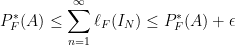
![J_n := I_n \cap (-\infty, t]](https://s0.wp.com/latex.php?latex=J_n+%3A%3D+I_n+%5Ccap+%28-%5Cinfty%2C+t%5D&bg=ffffff&fg=000000&s=0&c=20201002) and
and  ; note that
  and
and  cover
cover  and
and  , respectively. Also notice that
  . This gives us
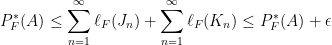
![\displaystyle \implies P_F^*(A) \leq P_F^*(A \cap (-\infty, t]) + P_F^*(A \cap (t, \infty)) \leq P_F^*(A) + \epsilon](https://s0.wp.com/latex.php?latex=%5Cdisplaystyle+%5Cimplies+P_F%5E%2A%28A%29+%5Cleq+P_F%5E%2A%28A+%5Ccap+%28-%5Cinfty%2C+t%5D%29+%2B+P_F%5E%2A%28A+%5Ccap+%28t%2C+%5Cinfty%29%29+%5Cleq+P_F%5E%2A%28A%29+%2B+%5Cepsilon&bg=ffffff&fg=000000&s=0&c=20201002)
![\displaystyle \implies P_F^*(A) = P_F^*(A \cap (-\infty, t]) + P_F^*(A \cap (-\infty, t]^\complement)](https://s0.wp.com/latex.php?latex=%5Cdisplaystyle+%5Cimplies+P_F%5E%2A%28A%29+%3D+P_F%5E%2A%28A+%5Ccap+%28-%5Cinfty%2C+t%5D%29+%2B+P_F%5E%2A%28A+%5Ccap+%28-%5Cinfty%2C+t%5D%5E%5Ccomplement%29&bg=ffffff&fg=000000&s=0&c=20201002)
 , is the distribution of some random variable.
 . We can measure the length of an interval
  in
in  and
and  (e.g.,
 ![{}[a, b]](https://s0.wp.com/latex.php?latex=%7B%7D%5Ba%2C+b%5D&bg=ffffff&fg=000000&s=0&c=20201002) ) as
) as .
. with the interval
 ![(a, b]](https://s0.wp.com/latex.php?latex=%28a%2C+b%5D&bg=ffffff&fg=000000&s=0&c=20201002) , but I believe this gives the same measure in the end.)
, but I believe this gives the same measure in the end.) , as follows.
 is a bounded interval. Proceeding as we would in defining the usual Lebesgue measure on
  be a measure on
  where
where

 , though with the standard Lebesgue measure we have
  .
.
 over
over  using the measure obtained from
  . We can create a new measure space
  where
where

 , and any other set
  is a subset of
  represents the probability of
  to be the probability of
  using the
  measure defined above. Of course, our measure and sigma-algebra are so simple that we can just write this in one line as
 given
given  , we say that

 implies
  . Plugging into the formula for
 .
. -algebra on


 is called a measure if it satisfies the properties


 we say that our triple is in fact a probability space. This is a formalization of our intuitive ideas of what a “probability space” should be — we have a set of all things that could conceivably happen (a sample space), a family of subsets of items from that sample space (events), and a way to assign a numerical value (a probability) to each of those events. The properties of a measure, in particular, aren’t particularly surprising in this context. If we have one event contained in another event, we’d expect the probability of the larger event to be greater than the probability of the smaller event; if we have a sequence of disjoint events, the probability at least one of them occurs is the sum of their probabilities; the probability something happens is one, and the probability nothing happens is zero.
 and
and  . When dealing with probabilities, we’re given that
  we have
  .
. ,
,  and
and  where
where  denotes the power set (the collection of all subsets) of
  is the cardinality of
  gives a measure where all events of the same size (cardinality) are equally likely.
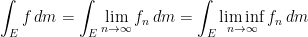
 is a sequence of non-negative measurable functions and
  increases monotonically to
  for each
  ,
,  pointwise (this can actually be relaxed to just having
  .
. a.e. for each
  , and so
  for each
  . Now also notice that since
  , that
  forms a bounded monotonic sequence sequence of real numbers, so it must converge. So we have
 is a Lebesgue measurable set and
 and
and  . Let
. Let  be a simple function with
  . Assume
  on
on  is trivial. Now define
  as follows.
 . Now note that
  and
and  , so there must exist an
  for all
  and notice that
  . Also,
  . For
. For  we have the following.


 this gives us

 , then we have
 as
as ![C_0 = [0, 1]](https://s0.wp.com/latex.php?latex=C_0+%3D+%5B0%2C+1%5D&bg=ffffff&fg=000000&s=0&c=20201002) . Then we construct
. Then we construct  from
from  by removing the middle third of
 ![C_1 = [0, 1/3] \cup [2/3, 1]](https://s0.wp.com/latex.php?latex=C_1+%3D+%5B0%2C+1%2F3%5D+%5Ccup+%5B2%2F3%2C+1%5D&bg=ffffff&fg=000000&s=0&c=20201002) . We then construct
. We then construct  by removing the middle third of the intervals in
 ![C_2 = [0, 1/9] \cup [2/9, 1/3] \cup [2/3, 7/9] \cup [8/9, 1]](https://s0.wp.com/latex.php?latex=C_2+%3D+%5B0%2C+1%2F9%5D+%5Ccup+%5B2%2F9%2C+1%2F3%5D+%5Ccup+%5B2%2F3%2C+7%2F9%5D+%5Ccup+%5B8%2F9%2C+1%5D&bg=ffffff&fg=000000&s=0&c=20201002) . In general, we will construct
. In general, we will construct  from
from  by removing the middle third of any interval in
 intervals (we start with
  intervals with
  . This means the sum total length of
 , we can find an
  , and so there exists an
  with
with  , and on the endpoints of intervals in each
  .)
.)